- Information
- AI Chat
Lecture Notes
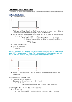
Statistics for business I (MA20228)
University of Bath
Students also viewed
- Statistics Coursework Report
- Notes - Question regarding leaving a partnership or terminating a partnership
- MA20225-sheet 6-2022 - help with exercise sheets for the given lecture notes and problems
- MA20225-sheet 5-2022 - help with exercise sheets for the given lecture notes and problems
- MA20225-sheet 4-2022 - help with exercise sheets for the given lecture notes and problems
- Heart Development and Defects
Preview text
10/02/
Pre lecture notes
lecture 1
random
exp
=
outcome
can't
be
predicted
with
certainty
can be
repeated
indefinitely
,
under
same
conditions
random variable
=
a
number
given
to each outcome
often
annotated
as
✗ or
Y
>
depends
how
many
RV's there are
make
quantitative
treatment
of
RE's
possible
RV is
often
capital
letter
,
the values of
RV
=
lower
case
>
symbol
convention
discrete RV
finite
number of
values
continuous RV
=
infinite
number of
values
(
probability
)
distribution
=
the
pattern
the RV
's
follow
normal
,
uniform
,
binomial
, Poisson
,
hypergeometric
distribution
for
DRV
=
✗
→
Pi
=
f-
Gci)
lgas
signs
probability
probability functions
valyespea.e
,
¥÷¥¥¥Ñ¥¥
(
specific
)
discrete
uniform distribution
=
finite
number
of
values are
equally
likely
to
be
observed
flock
In
e.
g. throwing
a
dice
> PCX -41=
,
PC✗=2)=Y
,
PCX-31= .. .
>
fG)=f
(2)
if
(3)
=fGD=fG)=fG)
Independent
random variables
= 2
variables
that aren't
correlated
correlation
between
RV
's ✗ andY
=
Pxx
> =
measures
linear
relationship
between 2 Variables
>
between
and
=
XP
,
YI * 2
IRV
'S
=
P✗Y=O
=
✗
F
,
YA but
1=
=
perfect
correlation PXY-
=/
2
IRV
's
0
no correlation
mean
aka
expected
value
of t/---ECXJ
Mean
of
prob
dist
=
μ✗=¥xifGc
;)
←
for
DRV
variance
= ok
-_
spread
of
Rv
around
μ
####### %¥¥£Éμ×B=§cxi
μ×Y
fix;)
""
Rules
i
mean
of
sum of
2 RVs
= sum of
means of
the individual RV
's
μ×+y= Mx
My
mean
of
the
product
of
RV and
a constant (a)
=
product
of
constant
and
mean of
RV
μ
ax
= a
Mx
:
μ✗ 2 ✗
=
2 ×μ✗
variance of
product
of
RV
by
constant
=
product
of
var of RV
and
square
of
constant
Otay
=
of0k
23/02/
Pre
lecture notes
lecture
2
Binomial Distribution
binomial
experiment
=
n
repeated
trials
,
with each
trial
having
2 outcomes
(
success or failure
)
PCs
)
=p
and
PCF )
= 1-
p
trials are
independent
binomial
RV
=
number of successful
outcomes
bbc.n
=
p41-p)n-x
x=number
of
successful
outcomes
a-
number
of
trials
p
probability
of
success
1%
number of
combinations
'
n
choose X
'
n
!
(E)
=
so :(n
x):
e.
g.
if
A-
4 and x=
:
4
!
2
! (4-2)
!
→
4 × 3 × 2 × 1
→
2 ¥
=
f
2 × 1 × 2 × 1
anything
choose 0=
☒
I choose 1
=
x
coin
example
=
coin
is
flipped
5
times
,
calculate
probability
distribution where
head
is success.
bloc :-b
,
)
(E)
pxc1-pln-xpb
)
=
(F)
0--1× 1 ×0=0.
Pfx= 1)
=
(7)
0.540=5×0× 0 -0625=0.
Pbc
:
=
(E)0.540=10×0×0--0.
PGc=
3)=
(3)0-512=10×0×025--
PCx= 47=(110-5)
'
=
5 ×0×0=0-
Pfx=5)=(
E.)
0-59=1×0×1--0.
mean
=
μ×=np
e.
g.
coin
example
:
μ×=
5 ×0-5--
variance
ok
=
npctp
)
e.
g.
coin
example
:
02--2-5×0=1.
binomial
proportion
=
number
of
successes
÷
number
of
trials
:
p= In
μp=p
o§=pa
pl
n
need
to calculate 2
values
z=
X
M
2cg
ample
)=fn
'
0
example
: time
taken
by
bus =
✗
,
mean
= 32 mins
,
var
=
100min
,
bus is late
if
it
takes
over
37 Mins .
What is
prob
bus
is
late
?
2--37-
=
51-0--0-
Foo
PIX >
37 )
=
Plz
>
0=
Plz e-
0%1-0-6915=
7
7
9
7
Pllate
)
Pllate
plnot late)
2 score at
05 on
2 table
= bus is
late 31%
of
times
B)
how
long
does slowest 20%
journeys
last
?
→
all
times
greater
than
xo
=
20%
slowest
PCX
>
xo)
= 0. so ☒
e-
Xo
)
=
→
on z
table
,
0=0.
so
,
DC -
=
0-
-1> 10 (0-84)-132=40.
10
=
20%
of
slowest
journeys
are
at least
404
mins
213122
pre
lecture notes lecture 3
Population
and sample
a
sample
is a small
part
of
population
population
full
set
of
individuals we want
to draw conclusions
from
sample
mean will
be
different
to
population
mean
different samples
have different means
I
=L
?§xi
=
'ñfX
,
-1×2+14....
- '
XD
Central
Limit Theorem
central
limit theorem
=
when
sample
size
is
large
cnzz
,
the
sampling
distribution
of
the
sample
mean
is
very
close to normal distribution
if
pop
.
mean
=
μ
,
and
pop
. var
= o?
the
sampling
distribution
of
sample
mean
=
I~NCM
example
:
Time taken
for
bus
journey
is norm
.
dist
. with
μ
-32mins
and
0=10 mins
.
One week
,
a sample
of
35
buses
gave
mean
of
335
.
A- 35
,
I
=
335
sampling
dist
of
E= 33 NC
,
¥1s)
→ INN
(32,1-69)
E)
z=✗¥✗n
=
335,2=13*
,
= 0.
=
0-
1- 0-
=
018943
Point Estimation lecture
4
recap
=
central
limit theorem
states
if
a
sample
size is above
30
,
Jc
is close
to
μ
,
and
§
is
close to
p
sample
variance
=s
5=?§(
Xi
- x-P
n
l
the S2 is
= 02 .
so
S2 is
a
point
estimator
for
02
>
5C is
point
estimator
for
μ
>
§
is
point
estimator
for p
parameter
point
estimator
M
ñ=¥
point
estimators are
helpful
when
parameter
is
02
5=?§CXi
- IT
Unknown
n
I
p
§
In
Interval
Estimation
used because
point
estimation
doesn't
provide
sufficient statistical
information
.
interval estimation uses
sample
data
to estimate
an
interval
of
possible
values
of
a
parameter
of
interest
point
est
only
gives
a
single
value
focusing
on
5C
Where n
>
30
I can have
any
value
,
but
it's
likely
dose to
μ
.
We want
to
quantify
this closeness
by
finding
an
interval Jc
and
μ
are
both in
¥¥'¥÷¥g
95%
probability
that distance
between Jc and
μ
is not
greater
i than distance between Xu or xrand
μ
"
÷
"
"
"
"
→
si.
probability
that
I is outside
shaded area
to
find
interval
of
951
.
confidence
.
Must
find
either
μ
Xe
or
Xr
M
4
>
these
lengths
are
identical to
I
Ice or Er
I
>
where Ir and
Ecu are
the
extremes of
the
interval we are
looking
for
5C
za
,
%sμ<
I
-12%
Ern
example
:
insurance
company
estimates
mean
age
of
policy
holders .
A
survey
of
36
samples
has mean
age
of
39s and variance of
What is
estimation
for
average age
at 90%
confidence
?
g-
fμz%nEμEÑ+t%%
two
, two tailed
.
00s one
tailed
df=
36-1=
895-4%
e-
ME
395+4%
3732M£
41-
Interval Estimation for
Proportion
use when
trying
to
find
a
proportion
within a
sample
⑧ -2%
a-
PED
-12%
example
:
⑧
~
Nlp ,
JET
☒
=
In
=
7*0=
o
=
if
=
=
034-1-96×0.
EPE
0341-1-96×0.
EPE
example
:
E- 2180
,
0=
,
n=3O
Ho
:p
-2000 vs Hi
:μ
✗
St.
=
Two
Sample Hypothesis Te s t i n g
: lecture
7
(6)
- 2
independent populations
example
:
30 CEO
's
.
12 women
and 18 men
showed
average salary
for
women was 76 million
and
average
salary
for
men was
- Million .
Means are
unknown
,
but
of
=
12
million
and on
.-1
.
Test at a-8.
critical
if
average
Womens
salary
differs
from
mens.
awe
I. ~N(
μ
,,
%-) Xin
Nlpk
,
%)
difference of
difference
-_
I
,
Ez~N(
μ
,
μ
,
o÷Y
sample
means
test
hypothesis
:
Ho
=
Mm
μf=O
Hi
=
Mm
Mf
=/
0
←
%n÷¥¥ =
E#--2-Hceo=MwdeepaidCV--
1-
214>1-
,
so
reject
tf
"
"
"
/
testtaistiu
Two
sample
testing
with unknown
and
equal
variances
when
the
population
variances are unknown we use
the
sample
standard deviations
G) and calculate
the mean
weight
.
The
mean
weight
is
called the
pooled
variance
estimate Gip
)
5p=
In
,
-11s
:
(
Nz
- Ps
N ,
- Nz -
We must use
the t
score .
E-
Ii-Ez_
szp%+ntÑ
the
CV
can
be
found
on table
where
DF
= At Nz
example
:
independent
random
samples of checking
account
balances
a
2 branches showed
:
Branch aNE-oud-ntssmaemakespsa ,
A
,
Yo
'
a
¥ 8
test at £-
.
It= 1000 ÑB
= 920
Sa
= 150 515-120 AA=
12 NB=lO
§p= (12-1)
is021-(10-1) 1202 = 18855
12+10-
t.io/z-7to--10oo-92O---
1 D.
F- 20
.
I sided test so E- oros
=
1-
FEE :o)
as
taboos ,
we can't
reject
null
hypothesis
.
When we
are
using
proportions
instead
of
means
,
we use
the
pooled probability
of success
④
⑤
=p ,§
, the$ 2
N
,
1- Nz
and the
pooled
variance
becomes
:
5-a
-0-(1-8)
ftp)
Lecture Notes
Module: Statistics for business I (MA20228)
University: University of Bath

- Discover more from:
Students also viewed
- Statistics Coursework Report
- Notes - Question regarding leaving a partnership or terminating a partnership
- MA20225-sheet 6-2022 - help with exercise sheets for the given lecture notes and problems
- MA20225-sheet 5-2022 - help with exercise sheets for the given lecture notes and problems
- MA20225-sheet 4-2022 - help with exercise sheets for the given lecture notes and problems
- Heart Development and Defects
